HVAC
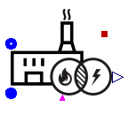
CHP
The CHP model is a performance-based model that assumes constant natural gas consumption and constant total efficiency. The electrical efficiency is described by the second-law efficiency and the efficiency of Carnot:
The second law efficiency is assumed constant and is defined by the previous equation at the nominal conditions. The electrical and thermal power are computed by:
where the thermal efficiency is described by:
The heat source is assumed to be at a constant temperature. The properties of the primary fluid are computed using the incompressible Cell1Dim model. The model includes a boolean input connector, which defines the operational state of the CHP, and a real output connector for the electrical power. In the equations, the boolean input is translated to the variable UONOFF.
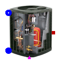
Heat Pump
This heat pump model does not consider part-load operation (ON/OFF regulation is assumed). The nominal heat flow is an input of the model, characteristic of the size of the heat pump. The COP is described by:
The second-law efficiency is assumed to remain unchanged in part-load operation. The electrical power consumed by the heat pump is described by:
In order to account for the lower heat capacity of the heat pump at lower evaporating temperature, the heating power and the heat soure temperature are computed by assuming a linear correlation between their actual and nominal values:
The primary fluid is modeled by means of 1-D incompressible fluid flow model (Cell1DimInc), in which a dynamic energy balance and static mass and momentum balances are applied on the fluid. The heat transfer in the primary fluid is modeled with a constant heat transfer coefficient. However, it can be changed to other heat transfer models through the HeatTransfer parameter in the fluid model.
Furthermore, the model includes a Boolean input connector on_off, which defines the operational state of the heat pump. In the equations, the Boolean input is translated to a variable value together with a first order block, which can take into account a start-up time constraint.
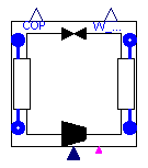
Heat Pump Consoclim
This model is used to determine the performances of a heat pump for different operating conditions. The ConsoClim model developed by the Ecole de Mines (Paris) is used. The model predicts the performances of the system with three polynomial laws. The parameters of the model are identified with manufacturer data.
The first and the second law (EIRFT and CAPFT) are used respectively to determine the COP and the heating capacity of the machine at full load. These two polynomial laws depend on the outside air temperature (T_a_out) and the temperature of the water at the exhaust of the condenser (T_w). The third law is used to determine the performances of the system at part load.
The primary side fluid is modeled by means of 1-D incompressible fluid flow model , in which a dynamic energy balance and static mass and momentum balances are applied on the fluid. The heat transfer in the primary fluid is modeled with a constant heat transfer coefficient. However, it can be changed to other heat transfer models through the HeatTransfer parameter in the fluid model.
Furthermore, the model includes a Boolean input connector on_off, which defines the operational state of the heat pump. In the equations, the Boolean input is translated to a variable value together with a first order block, which can take into account a start-up time constraint. The model also includes a real input connector W_dot_set to define the power that is injected to the heat pump. This connector is useful, for example, in the case where a heat pump is powered by the CHP electrical generation.
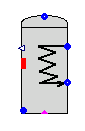
Thermal energy storage
Nodal model of a stratified tank with an internal heat exchanger and ambient heat losses. The following hypothesis are applied:
- No heat transfer between the different nodes.
- The internal heat exchanger is discretized in the same way as the tank: each cell of the heat exchanger corresponds to one cell of the tank and exchanges heat with that cell only.
- Incompressible fluid in bboth the tank and the heat exchanger.
The tank is discretized using a modified version of the incompressible Cell1Dim model adding an additional heat port, which acts as a heating resistance. The model also includes a temperature sensor, whose height can be adjusted. The energy balance of the fluid in the tank is described by:
The heat exchanger is modeled using the Flow1Dim component and a wall component. The energy balance of the fluid in the heat exchanger is described by: